The Distribution of Cherry Trees in Washington DC

1 Introduction

I had long wished to see cherry blossom in Washington DC. However, this year has been a year of staying in, which makes me even more eager to see it. As a result, I pulled up cherry trees data from the open data portal and explored it before I can see it in person. In this notebook, I will first use ggplot2 to map the cherry data and then play with leaflet to try the interactive visualization.

2 Data Preparation

2.1 Set Up

knitr::opts_chunk$set(echo = TRUE, fig.align = "center")
library(leaflet) 
library(tidyverse)
library(funModeling) 
library(readr)
library(rgdal) 
library(hexbin)

2.2 Read in data and clean

trees <- read_csv("Urban_Forestry_Street_Trees.csv")
head(trees)

## # A tibble: 6 x 39
##       X     Y OBJECTID FACILITYID VICINITY  WARD TBOX_L TBOX_W WIRES CURB  SIDEWALK TBOX_STAT
##   <dbl> <dbl>    <dbl> <chr>      <chr>    <dbl>  <dbl>  <dbl> <chr> <chr> <chr>    <chr>    
## 1 -77.0  38.9 43998460 10110-185~ 1810 11~     1      9      4 None  Perm~ Permane~ Plant    
## 2 -77.0  38.9 43998509 <NA>       2200 BL~     6     99      9 None  None  None     Plant    
## 3 -77.0  38.9 43998510 28801-200~ 2000 UP~     5     99      3 Both  Perm~ Permane~ Plant    
## 4 -77.1  38.9 43998511 10393-230~ 2408 39~     3     99      4 None  Perm~ Permane~ Plant    
## 5 -77.0  38.9 43998512 <NA>       2200 BL~     6     99      9 None  None  None     Plant    
## 6 -77.0  38.9 43998513 36981-290~ 2927 PE~     7     99      6 Both  Perm~ Permane~ Plant    
## # ... with 27 more variables: RETIREDDT <chr>, SCI_NM <chr>, CMMN_NM <chr>, DATE_PLANT <chr>,
## #   DBH <dbl>, DISEASE <chr>, PESTS <chr>, CONDITION <chr>, CONDITIODT <chr>, OWNERSHIP <chr>,
## #   TREE_NOTES <chr>, ONEYEARPHOTO <chr>, SPECIALPHOTO <lgl>, PHOTOREMARKS <lgl>,
## #   ELEVATION <chr>, SIGN <chr>, TRRS <dbl>, WARRANTY <chr>, FAM_NAME <chr>, CREATED_USER <chr>,
## #   CREATED_DATE <chr>, EDITEDBY <chr>, LAST_EDITED_USER <chr>, LAST_EDITED_DATE <chr>,
## #   GENUS_NAME <chr>, GLOBALID <chr>, SHAPE <lgl>

df_status(trees)

##            variable q_zeros p_zeros   q_na   p_na q_inf p_inf      type unique
## 1                 X       0    0.00      2   0.00     0     0   numeric 190378
## 2                 Y       0    0.00      2   0.00     0     0   numeric 190380
## 3          OBJECTID       0    0.00      0   0.00     0     0   numeric 190769
## 4        FACILITYID       3    0.00  38324  20.09     0     0 character 149091
## 5          VICINITY       0    0.00   3404   1.78     0     0 character 115842
## 6              WARD       0    0.00    766   0.40     0     0   numeric      8
## 7            TBOX_L      20    0.01  17801   9.33     0     0   numeric     99
## 8            TBOX_W      24    0.01  17763   9.31     0     0   numeric     81
## 9             WIRES       0    0.00   3467   1.82     0     0 character      4
## 10             CURB       0    0.00   3311   1.74     0     0 character      4
## 11         SIDEWALK       0    0.00   3453   1.81     0     0 character      4
## 12        TBOX_STAT       0    0.00     95   0.05     0     0 character      8
## 13        RETIREDDT       0    0.00      0   0.00     0     0 character   4305
## 14           SCI_NM       0    0.00  15951   8.36     0     0 character    206
## 15          CMMN_NM       0    0.00  14971   7.85     0     0 character    205
## 16       DATE_PLANT       0    0.00      0   0.00     0     0 character  43530
## 17              DBH    4714    2.47  15785   8.27     0     0   numeric    603
## 18          DISEASE       0    0.00 188871  99.01     0     0 character     11
## 19            PESTS       0    0.00 189673  99.43     0     0 character      5
## 20        CONDITION       0    0.00  14881   7.80     0     0 character      5
## 21       CONDITIODT       0    0.00      0   0.00     0     0 character 153216
## 22        OWNERSHIP       0    0.00   1135   0.59     0     0 character      7
## 23       TREE_NOTES       7    0.00 115204  60.39     0     0 character  34001
## 24     ONEYEARPHOTO       0    0.00 189991  99.59     0     0 character     28
## 25     SPECIALPHOTO       0    0.00 190768 100.00     0     0   logical      1
## 26     PHOTOREMARKS       0    0.00 190769 100.00     0     0   logical      0
## 27        ELEVATION     245    0.13  11773   6.17     0     0 character      7
## 28             SIGN       0    0.00  12744   6.68     0     0 character      6
## 29             TRRS      53    0.03 190431  99.82     0     0   numeric     11
## 30         WARRANTY       0    0.00  24317  12.75     0     0 character     17
## 31         FAM_NAME       0    0.00  20812  10.91     0     0 character     86
## 32     CREATED_USER       0    0.00 151684  79.51     0     0 character     38
## 33     CREATED_DATE       0    0.00      0   0.00     0     0 character  34899
## 34         EDITEDBY       0    0.00   5648   2.96     0     0 character     40
## 35 LAST_EDITED_USER       0    0.00     19   0.01     0     0 character     40
## 36 LAST_EDITED_DATE       0    0.00      0   0.00     0     0 character 152696
## 37       GENUS_NAME       0    0.00  25420  13.33     0     0 character     77
## 38         GLOBALID       0    0.00      0   0.00     0     0 character 190769
## 39            SHAPE       0    0.00 190769 100.00     0     0   logical      0

Rename variables to meaningful names and filter out rows that lack longitude or latitude.

trees <- trees %>% 
  rename(long= X, lat=Y, plant_names=CMMN_NM) %>% 
  filter(!is.na(long) & !is.na(lat) & !is.na(plant_names))

Filter trees that has “cherry” in the plant names.

cherry_trees <- trees %>% 
  filter(str_detect(trees$plant_names, regex(".*cherry.*", ignore_case=TRUE))) %>% 
  select(long, lat, plant_names)

Now we have the cherry data, we would like to see the cultivars and the quantity of each cultivar.

cherry_trees %>% 
  count(plant_names) %>% 
  arrange(desc(n))

## Warning: `...` is not empty.
## 
## We detected these problematic arguments:
## * `needs_dots`
## 
## These dots only exist to allow future extensions and should be empty.
## Did you misspecify an argument?

## # A tibble: 7 x 2
##   plant_names            n
##   <chr>              <int>
## 1 Cherry              2209
## 2 Kwanzan cherry      2038
## 3 Chokecherry         1929
## 4 Yoshino cherry      1835
## 5 Cherry (Snowgoose)  1813
## 6 Okame cherry         855
## 7 Cherrybark Oak         5

The most common cultivar is cherry without explicitly identifying its cultivar. There’s no other evidence here that would help us determine what it is, so we will just go with its original name- Cherry. In addition, after a bit of googling, it turns out that Cherrybark Oak is not a cherry tree, although it has cherry in its name. Thus I will exclude that from the data and in the meantime, update Chokecherry and Cherry (Snowgoose) to make all of the names have the same pattern.

cherry_trees <-  cherry_trees %>% 
  filter(plant_names!="Cherrybark Oak") %>% 
  mutate(plant_names=case_when(.$plant_names=="Chokecherry" ~ "Choke cherry",
                               .$plant_names =="Cherry (Snowgoose)" ~ "Snowgoose cherry",
                               TRUE ~ .$plant_names
                              ))

Up till now the cherry tree data is ready. To map the cherry tree location to the map of DC, we need a DC map with neighborhoods boundaries.

2.3 DC shapefile

Read in the shapefile using rgdal package.

#create a folder to hold the dc shape files
dir.create("dc_shape1")
unzip("Neighborhood_Clusters-shp.zip", exdir = "dc_shape1")

#read in the dc shape file 
shp <- readOGR("dc_shape1/Neighborhood_Clusters.shp")

## OGR data source with driver: ESRI Shapefile 
## Source: "C:\Users\wensh\Desktop\dccherrytrees\dc_shape1\Neighborhood_Clusters.shp", layer: "Neighborhood_Clusters"
## with 46 features
## It has 7 fields

Now both of the cherry tree and map data are ready, it is time to plot them out and see the distribution of the cherry.

3 Data Visualization

3.1 ggplot2 Basic visualization

ggplot()+geom_polygon(data=shp, aes(long, lat, group=group), colour="black", fill=NA)+geom_point(data=cherry_trees, aes(long, lat))+theme_void()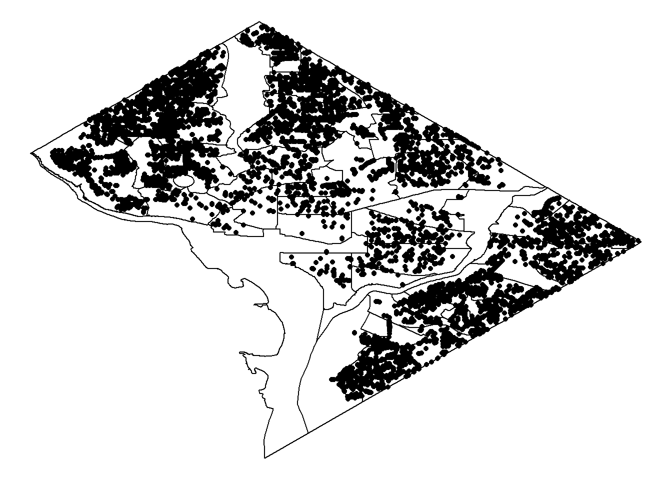

The basic visualization is hard to detect the number of trees in the communities. Hex geom can better plot the density. In the following, I will change the geom to hex and the colour scheme to fit in the cherry blossom atmosphere!

3.1.1 Geom and Color Change

p <- ggplot()+geom_polygon(data=shp, aes(long, lat, group=group), colour="black", fill=NA)+
  geom_hex(data=cherry_trees, aes(long, lat))+
  scale_fill_gradient(name="No. of trees", low="#ffcee6", high = "#6B0772")+theme_void()
print(p)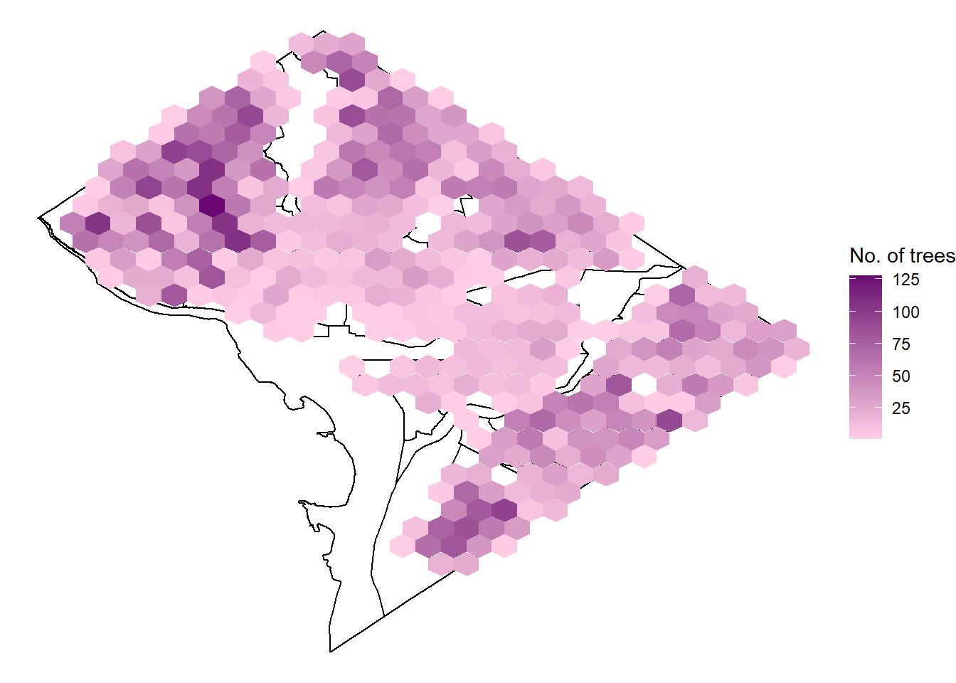

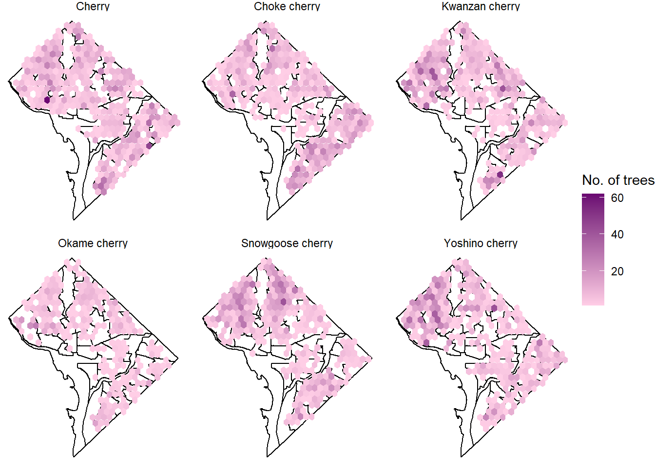
3.1.2 Distribution of Different Cultivars

Sometimes people have their preference when it comes to what kind of cherry trees to see, here I will subset the trees by facet_wrap() so people will know where to go based on the type of trees they prefer.

p <- p+facet_wrap(~plant_names)
print(p)

# customize the plots

p+labs(title=" The Distribution of Cherry Trees in Washington DC", 
       caption="data source: Open Data DC 2020")+
   theme(plot.title=element_text(hjust = 0.5, margin=margin(b=16)), 
        legend.position = "bottom", legend.direction = "horizontal", 
        legend.title = element_text(vjust=0.9, size = 8), 
        legend.text = element_text(size=8), 
        legend.box.spacing = unit(1, "cm"),
        legend.key.size = unit(4, "mm"),
        plot.caption = element_text(face = "italic", color = "#696969"))

I tried to add the neighborhoods names to the plots but it made the plots a mess. Next I will try to utilize leaflet package to build an interactive map with the neighborhoods names shown on the map.

3.2 Interactive visualization

3.2.1 DC Interactive map with neighborhood names shown

First, I will use DC shape data shp to create an interactive map where you can see the corresponding neighborhood names when hovering over.

leaflet() %>% 
  addTiles() %>% 
  addPolygons(data=shp,
              label = ~NBH_NAMES,
              color = "444444",
              weight=1,
              smoothFactor = 0.5,
              opacity = 1.0,
              fillOpacity = 0.5,
              highlightOptions = highlightOptions(color = "white",
                                                  weight = 2,
                                                  bringToFront = TRUE))

3.2.2 Cherry Data Added to the Map

Next, cherry data will be added as another layer to the map.

leaflet() %>% 
  addTiles() %>% 
  addPolygons(data=shp,
              label = ~NBH_NAMES,
              color = "444444",
              weight=1,
              smoothFactor = 0.5,
              opacity = 1.0,
              fillOpacity = 0.5,
              highlightOptions = highlightOptions(color = "white",
                                                  weight = 2,
                                                  bringToFront = TRUE)) %>% 
  addMarkers(data=cherry_trees, clusterOptions = markerClusterOptions())

A few places we can tell from the map are good for appreciation of cherry blossom: Twining, Cleveland Park, Brightwood Park and Congress Heights.

3.2.3 Seprate Maps for Different Cultivars

For people who have specific interests in certain kinds of cherry trees, below are the plots subsetting from the main one based on the type of cherry trees.

Cherry

leaflet() %>% 
  addTiles() %>% 
  addPolygons(data=shp,
              label = ~NBH_NAMES,
              color = "444444",
              weight=1,
              smoothFactor = 0.5,
              opacity = 1.0,
              fillOpacity = 0.5,
              highlightOptions = highlightOptions(color = "white",
                                                  weight = 2,
                                                  bringToFront = TRUE)) %>% 
  addMarkers(data=cherry_trees %>% filter(plant_names=="Cherry"), 
             clusterOptions = markerClusterOptions())

Places like Twinging, Brightwood Park and Brookland are densely distributed with Cherry.

Yoshino cherry

leaflet() %>% 
  addTiles() %>% 
  addPolygons(data=shp,
              label = ~NBH_NAMES,
              color = "444444",
              weight=1,
              smoothFactor = 0.5,
              opacity = 1.0,
              fillOpacity = 0.5,
              highlightOptions = highlightOptions(color = "white",
                                                  weight = 2,
                                                  bringToFront = TRUE)) %>% 
  addMarkers(data=cherry_trees %>% filter(plant_names=="Yoshino cherry"), 
             clusterOptions = markerClusterOptions())

Clearly, Yoshino cherry trees are more densely grown in the northwest of the city. More specifically, Friendship Heights is the place with most Yoshino.

Choke cherry

leaflet() %>% 
  addTiles() %>% 
  addPolygons(data=shp,
              label = ~NBH_NAMES,
              color = "444444",
              weight=1,
              smoothFactor = 0.5,
              opacity = 1.0,
              fillOpacity = 0.5,
              highlightOptions = highlightOptions(color = "white",
                                                  weight = 2,
                                                  bringToFront = TRUE)) %>% 
  addMarkers(data=cherry_trees %>% filter(plant_names=="Choke cherry"), 
             clusterOptions = markerClusterOptions())

People who have an penchant for Choke cherry should go to the east and southeast of DC. Places like Sheridan and Deanwood are good for Choke cherry.

Kwanzan cherry

leaflet() %>% 
  addTiles() %>% 
  addPolygons(data=shp,
              label = ~NBH_NAMES,
              color = "444444",
              weight=1,
              smoothFactor = 0.5,
              opacity = 1.0,
              fillOpacity = 0.5,
              highlightOptions = highlightOptions(color = "white",
                                                  weight = 2,
                                                  bringToFront = TRUE)) %>% 
  addMarkers(data=cherry_trees %>% filter(plant_names=="Kwanzan cherry"), 
             clusterOptions = markerClusterOptions())

Most of the Kwanzan cherry are located in the west of DC. If people go to Spring Valley and Friendship Heights, they should have a blast at the Kwanzan cherry.

Snowgoose cherry

leaflet() %>% 
  addTiles() %>% 
  addPolygons(data=shp,
              label = ~NBH_NAMES,
              color = "444444",
              weight=1,
              smoothFactor = 0.5,
              opacity = 1.0,
              fillOpacity = 0.5,
              highlightOptions = highlightOptions(color = "white",
                                                  weight = 2,
                                                  bringToFront = TRUE)) %>% 
  addMarkers(data=cherry_trees %>% filter(plant_names=="Snowgoose cherry"), 
             clusterOptions = markerClusterOptions())

If you are a big fan of Snowgoose cherry, you know where you should go- Cleveland Park, Friendship Heights, Brightwood Park and Takoma!

Okame cherry

leaflet() %>% 
  addTiles() %>% 
  addPolygons(data=shp,
              label = ~NBH_NAMES,
              color = "444444",
              weight=1,
              smoothFactor = 0.5,
              opacity = 1.0,
              fillOpacity = 0.5,
              highlightOptions = highlightOptions(color = "white",
                                                  weight = 2,
                                                  bringToFront = TRUE)) %>% 
  addMarkers(data=cherry_trees %>% filter(plant_names=="Okame cherry"), 
             clusterOptions = markerClusterOptions())

The west side of DC boasts the most Okame cherry trees. Spring Valley, Friendship Heights and Takoma are great to see Okame.

When the next cherry blossom season sets in, I hope you have an idea where you want to go for the best experience!